Effects.jl
Regression models are useful but they can be tricky to interpret. Variable centering and contrast coding can obscure the meaning of main effects. Interaction terms, especially higher order ones, only increase the difficulty of interpretation. Here, we introduce Effects.jl which translates the fitted model, including estimated uncertainty, back into data space. Using Effects.jl, it is possible to generate effects plots that enable rapid visualization and interpretation of regression models.
The examples below demonstrate the use of Effects.jl with GLM.jl, but they will work with any modeling package that is based on the StatsModels.jl formula. The second example is borrowed in no small part from StandardizedPredictors.jl.
The Effect of Contrast Coding
Let's consider a synthetic dataset of weights (in grams) for chicks feed different types of feed, with a single predictor feed (categorical, with three levels A, B, C). The simulated weights are based loosely on the R dataset chickwts.
using AlgebraOfGraphics, CairoMakie, DataFrames, Effects, GLM, StatsModels, StableRNGs
rng = StableRNG(42)
reps = 5
sd = 50
wtdat = DataFrame(; feed=repeat(["A", "B", "C"], inner=reps),
                  weight=[180 .+ sd * randn(rng, reps);
                          220 .+ sd * randn(rng, reps);
300 .+ sd * randn(rng, reps)])| Row | feed | weight |
|---|---|---|
| String | Float64 | |
| 1 | A | 146.487 |
| 2 | A | 202.356 |
| 3 | A | 248.682 |
| 4 | A | 245.477 |
| 5 | A | 186.304 |
| 6 | B | 254.197 |
| 7 | B | 169.04 |
| 8 | B | 180.324 |
| 9 | B | 308.736 |
| 10 | B | 284.867 |
| 11 | C | 217.807 |
| 12 | C | 339.722 |
| 13 | C | 234.517 |
| 14 | C | 298.147 |
| 15 | C | 353.616 |
If we fit a linear model to this data using default treatment/dummy coding, then the coefficient corresponding of feed C is significant.
mod_treat = lm(@formula(weight ~ 1 + feed), wtdat)StatsModels.TableRegressionModel{GLM.LinearModel{GLM.LmResp{Vector{Float64}}, GLM.DensePredChol{Float64, LinearAlgebra.CholeskyPivoted{Float64, Matrix{Float64}, Vector{Int64}}}}, Matrix{Float64}}
weight ~ 1 + feed
Coefficients:
───────────────────────────────────────────────────────────────────────
Coef. Std. Error t Pr(>|t|) Lower 95% Upper 95%
───────────────────────────────────────────────────────────────────────
(Intercept) 205.861 25.075 8.21 <1e-05 151.227 260.495
feed: B 33.5719 35.4614 0.95 0.3625 -43.6919 110.836
feed: C 82.9008 35.4614 2.34 0.0375 5.63696 160.165
───────────────────────────────────────────────────────────────────────If on the other hand, we use effects (sum-to-zero) coding, then the coefficient for feed C is no longer significant:
mod_eff = lm(@formula(weight ~ 1 + feed), wtdat; contrasts=Dict(:feed => EffectsCoding()))StatsModels.TableRegressionModel{GLM.LinearModel{GLM.LmResp{Vector{Float64}}, GLM.DensePredChol{Float64, LinearAlgebra.CholeskyPivoted{Float64, Matrix{Float64}, Vector{Int64}}}}, Matrix{Float64}}
weight ~ 1 + feed
Coefficients:
──────────────────────────────────────────────────────────────────────────
Coef. Std. Error t Pr(>|t|) Lower 95% Upper 95%
──────────────────────────────────────────────────────────────────────────
(Intercept) 244.685 14.4771 16.90 <1e-09 213.143 276.228
feed: B -5.25232 20.4737 -0.26 0.8019 -49.8606 39.356
feed: C 44.0766 20.4737 2.15 0.0524 -0.531742 88.6849
──────────────────────────────────────────────────────────────────────────This is in some sense unsurprising: the different coding schemes correspond to different hypotheses. In treatment coding, the hypothesis for the coefficient feed: C is whether feed C differs from the reference level, feed A. In effects coding, the hypothesis is whether feed C differs from the mean across all levels. In more complicated models, the hypotheses being tested – especially for interaction terms – can become more complex and difficult to "read off" from the model summary.
In spite of these differences, these models make the same predictions about the data:
fitted(mod_treat) ≈ fitted(mod_eff)trueAt a deep level, these models are the actually same model, but with different parameterizations. In order to get a better view about what a model is saying about the data, abstracted away from the parameterization, we can see what the model looks like in data space. For that, we can use Effects.jl to generate the effects that the model is capturing. We do this by specifying a (subset of the) design and creating a reference grid, then computing the model's prediction and associated error at those values.
The effects function will compute the reference grid for a crossed design specified by a dictionary of values. As we only have one predictor in this dataset, the design is completely crossed.
design = Dict(:feed => unique(wtdat.feed))
eff_feed = effects(design, mod_eff)| Row | feed | weight | err | lower | upper |
|---|---|---|---|---|---|
| String | Float64 | Float64 | Float64 | Float64 | |
| 1 | A | 205.861 | 25.075 | 180.786 | 230.936 |
| 2 | B | 239.433 | 25.075 | 214.358 | 264.508 |
| 3 | C | 288.762 | 25.075 | 263.687 | 313.837 |
The effects table consists of four columns: the levels of the feed predictor specified in the design (feed), the prediction of the model at those levels (weight), the standard error of those predictions err, and the lower and upper edges of confidence interval of those predictions (lower, upper; computed using a normal approximation based on the standard error).
Because the effects are on the data (response) scale, they are invariant to parameterization:
effects(design, mod_treat)| Row | feed | weight | err | lower | upper |
|---|---|---|---|---|---|
| String | Float64 | Float64 | Float64 | Float64 | |
| 1 | A | 205.861 | 25.075 | 180.786 | 230.936 |
| 2 | B | 239.433 | 25.075 | 214.358 | 264.508 |
| 3 | C | 288.762 | 25.075 | 263.687 | 313.837 |
We can also compute effects on a subset of the levels in the data:
effects(Dict(:feed => ["A"]), mod_eff)| Row | feed | weight | err | lower | upper |
|---|---|---|---|---|---|
| String | Float64 | Float64 | Float64 | Float64 | |
| 1 | A | 205.861 | 25.075 | 180.786 | 230.936 |
Note that in this case, we computed the average effect of the level A, which is not directly encoded in any single model coefficient in this parameterization / contrast coding.
We can of course use the estimated effects to get a nice visual of the data:
plt = data(eff_feed) * mapping(:feed, :weight) * (visual(Scatter) + mapping(:err) * visual(Errorbars))
draw(plt)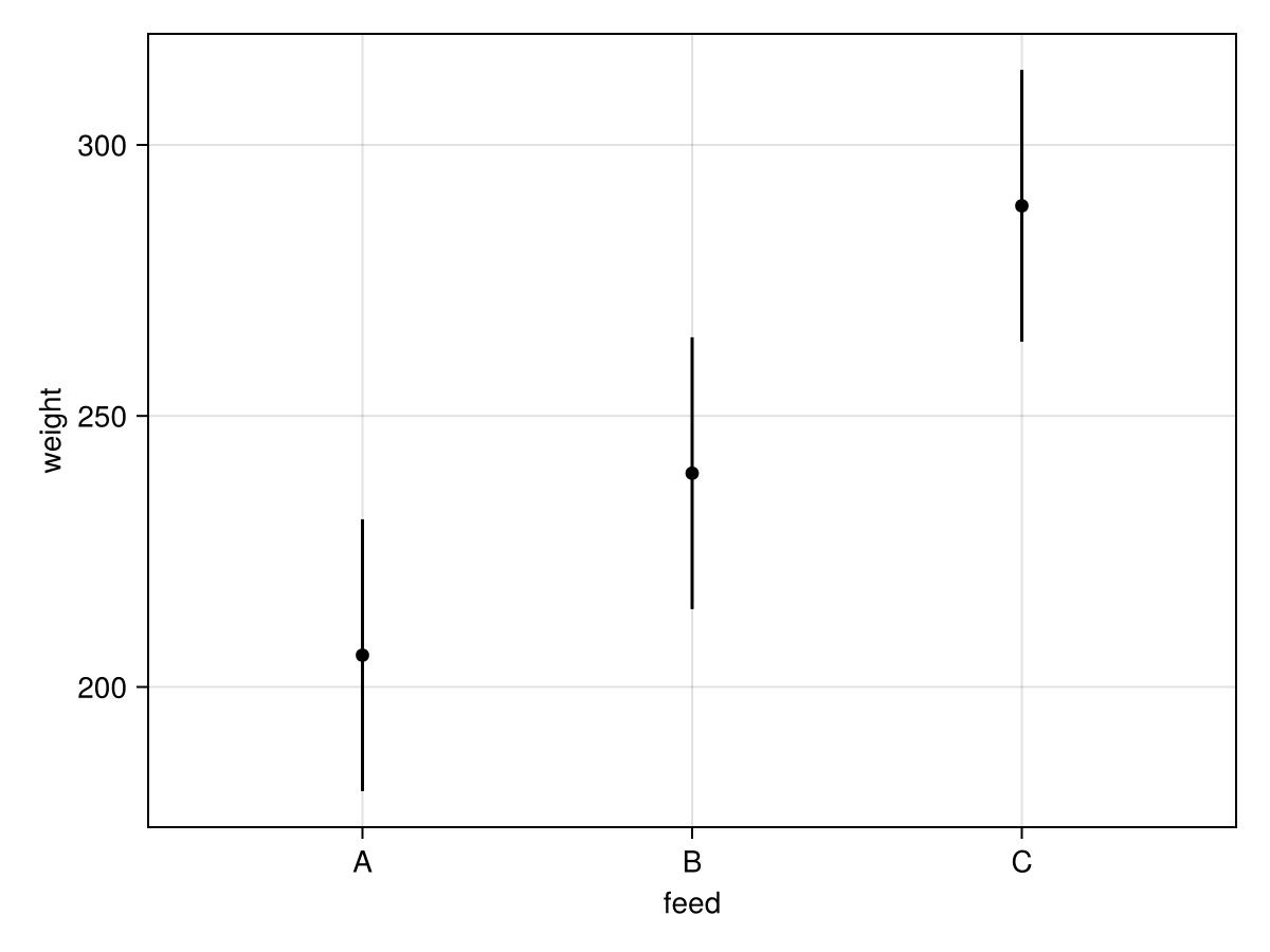
Interaction Terms in Effects
Let's consider a (slightly) synthetic dataset of weights for adolescents of different ages, with predictors age (continuous, from 13 to 20) and sex, and weight in pounds. The weights are based loosely on the medians from the CDC growth charts, which show that the median male and female both start off around 100 pounds at age 13, but by age 20 the median male weighs around 155 pounds while the median female weighs around 125 pounds.
using AlgebraOfGraphics, CairoMakie, DataFrames, Effects, GLM, StatsModels, StableRNGs
rng = StableRNG(42)
growthdata = DataFrame(; age=[13:20; 13:20],
                       sex=repeat(["male", "female"], inner=8),
weight=[range(100, 155; length=8); range(100, 125; length=8)] .+ randn(rng, 16))| Row | age | sex | weight |
|---|---|---|---|
| Int64 | String | Float64 | |
| 1 | 13 | male | 99.3297 |
| 2 | 14 | male | 108.304 |
| 3 | 15 | male | 117.088 |
| 4 | 16 | male | 124.881 |
| 5 | 17 | male | 131.555 |
| 6 | 18 | male | 139.97 |
| 7 | 19 | male | 146.124 |
| 8 | 20 | male | 154.206 |
| 9 | 13 | female | 101.775 |
| 10 | 14 | female | 104.869 |
| 11 | 15 | female | 105.499 |
| 12 | 16 | female | 111.509 |
| 13 | 17 | female | 112.976 |
| 14 | 18 | female | 117.82 |
| 15 | 19 | female | 122.501 |
| 16 | 20 | female | 124.603 |
In this dataset, there's obviously a main effect of sex: males are heavier than females for every age except 13 years. But if we run a basic linear regression, we see something rather different:
mod_uncentered = lm(@formula(weight ~ 1 + sex * age), growthdata)StatsModels.TableRegressionModel{GLM.LinearModel{GLM.LmResp{Vector{Float64}}, GLM.DensePredChol{Float64, LinearAlgebra.CholeskyPivoted{Float64, Matrix{Float64}, Vector{Int64}}}}, Matrix{Float64}}
weight ~ 1 + sex + age + sex & age
Coefficients:
──────────────────────────────────────────────────────────────────────────────
Coef. Std. Error t Pr(>|t|) Lower 95% Upper 95%
──────────────────────────────────────────────────────────────────────────────
(Intercept) 56.4387 2.88762 19.55 <1e-09 50.1471 62.7303
sex: male -56.1509 4.08372 -13.75 <1e-07 -65.0485 -47.2532
age 3.40941 0.173344 19.67 <1e-09 3.03172 3.78709
sex: male & age 4.31146 0.245146 17.59 <1e-09 3.77734 4.84559
──────────────────────────────────────────────────────────────────────────────Is this model just a poor fit to the data? We can plot the effects and see that's not the case. For example purposes, we'll create a reference grid that does not correspond to a fully balanced design and call effects! to insert the effects-related columns. In particular, we'll take odd ages for males and even ages for females.
refgrid = copy(growthdata)
filter!(refgrid) do row
    return mod(row.age, 2) == (row.sex == "male")
end
effects!(refgrid, mod_uncentered)| Row | age | sex | weight | err |
|---|---|---|---|---|
| Int64 | String | Float64 | Float64 | |
| 1 | 13 | male | 100.659 | 0.72515 |
| 2 | 15 | male | 116.101 | 0.474722 |
| 3 | 17 | male | 131.543 | 0.406528 |
| 4 | 19 | male | 146.984 | 0.587838 |
| 5 | 14 | female | 104.17 | 0.587838 |
| 6 | 16 | female | 110.989 | 0.406528 |
| 7 | 18 | female | 117.808 | 0.474722 |
| 8 | 20 | female | 124.627 | 0.72515 |
Note that the column corresponding to the response variable weight has been overwritten with the effects prediction and that only the standard error is provided: the effects! method does less work than the effects convenience method.
We can add the confidence interval bounds in and plot our predictions:
refgrid[!, :lower] = @. refgrid.weight - 1.96 * refgrid.err
refgrid[!, :upper] = @. refgrid.weight + 1.96 * refgrid.err
sort!(refgrid, [:age])

plt = data(refgrid) * mapping(:age; color=:sex) *
      (mapping(:weight) * visual(Lines) +
       mapping(:lower, :upper) * visual(Band; alpha=0.3))
draw(plt)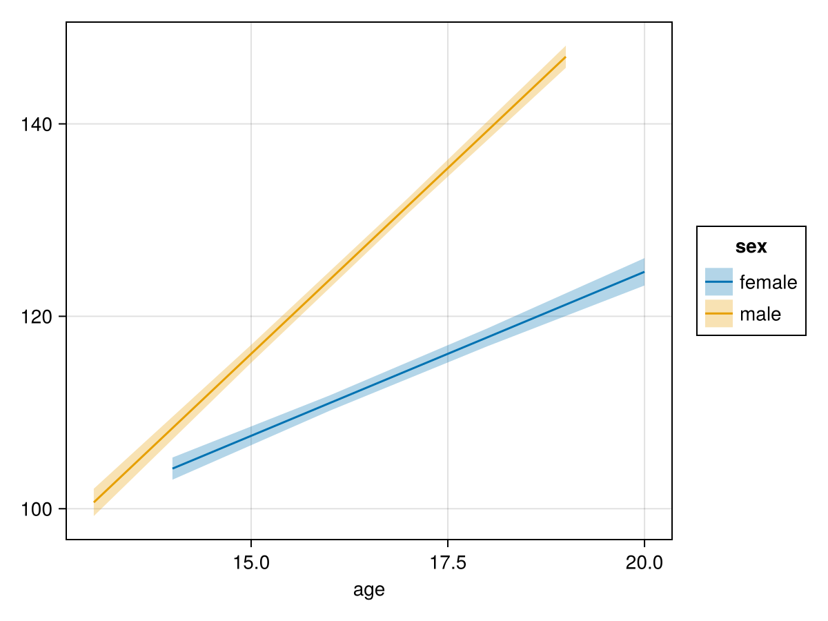
We can also add in the raw data to check the model fit:
draw(plt + data(growthdata) * mapping(:age, :weight; color=:sex) * visual(Scatter))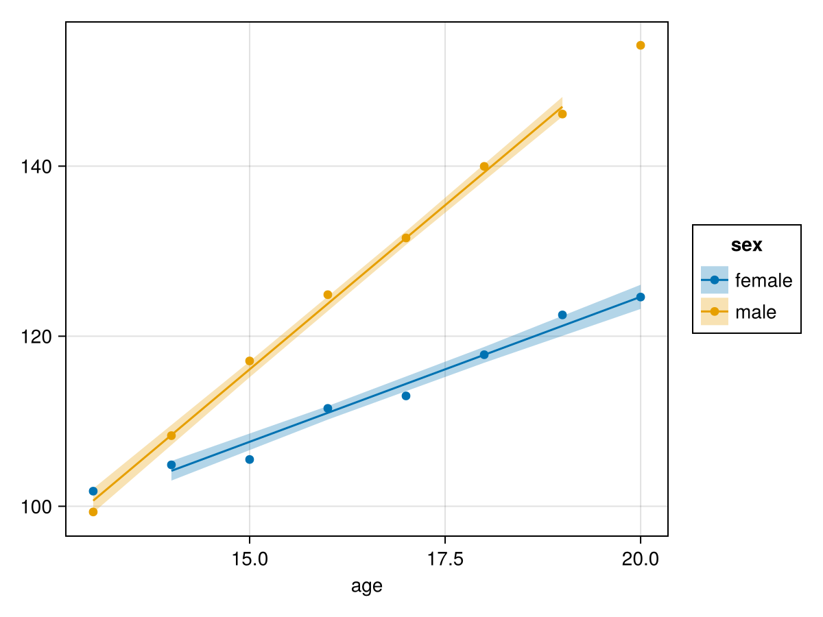
The model seems to be doing a good job. Indeed it is, and as pointed out in the StandardizedPredictors.jl docs, the problem is that we should center the age variable. While we're at it, we'll also set the contrasts for sex to be effects coded.
using StandardizedPredictors
contrasts = Dict(:age => Center(15), :sex => EffectsCoding())
mod_centered = lm(@formula(weight ~ 1 + sex * age), growthdata; contrasts=contrasts)
StatsModels.TableRegressionModel{GLM.LinearModel{GLM.LmResp{Vector{Float64}}, GLM.DensePredChol{Float64, LinearAlgebra.CholeskyPivoted{Float64, Matrix{Float64}, Vector{Int64}}}}, Matrix{Float64}}
weight ~ 1 + sex + age(centered: 15) + sex & age(centered: 15)
Coefficients:
────────────────────────────────────────────────────────────────────────────────────────────
Coef. Std. Error t Pr(>|t|) Lower 95% Upper 95%
────────────────────────────────────────────────────────────────────────────────────────────
(Intercept) 111.84 0.335679 333.18 <1e-24 111.109 112.572
sex: male 4.26052 0.335679 12.69 <1e-07 3.52914 4.99191
age(centered: 15) 5.56514 0.122573 45.40 <1e-14 5.29808 5.8322
sex: male & age(centered: 15) 2.15573 0.122573 17.59 <1e-09 1.88867 2.42279
────────────────────────────────────────────────────────────────────────────────────────────All of the estimates have now changed because the parameterization is completely different, but the predictions and thus the effects remain unchanged:
refgrid_centered = copy(growthdata)
effects!(refgrid_centered, mod_centered)
refgrid_centered[!, :lower] = @. refgrid_centered.weight - 1.96 * refgrid_centered.err
refgrid_centered[!, :upper] = @. refgrid_centered.weight + 1.96 * refgrid_centered.err
sort!(refgrid_centered, [:age])

plt = data(refgrid_centered) * mapping(:age; color=:sex) *
       (mapping(:weight) * visual(Lines) +
        mapping(:lower, :upper) * visual(Band, alpha=0.3))
draw(plt)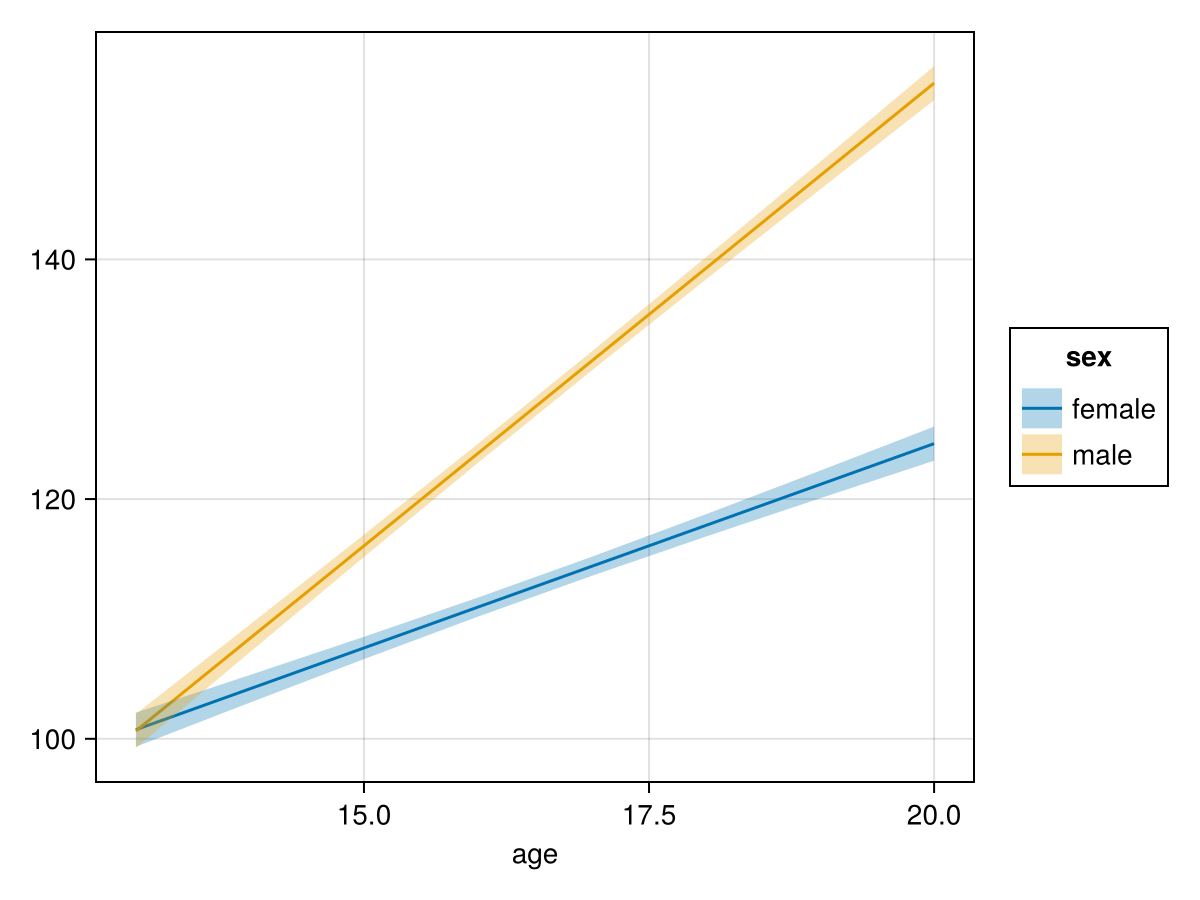
Understanding lower-level terms in the presence of interactions can be particularly tricky, and effect plots are also useful for this. For example, if we want to examine the effect of sex at a typical age, then we would need some way to reduce age to typical values. By default, effects[!] will take use the mean of all model terms not specified in the effects formula as representative values. Looking at sex, we see that
design = Dict(:sex => unique(growthdata.sex))
effects(design, mod_uncentered)| Row | sex | weight | err | lower | upper |
|---|---|---|---|---|---|
| String | Float64 | Float64 | Float64 | Float64 | |
| 1 | male | 127.682 | 0.397181 | 127.285 | 128.079 |
| 2 | female | 112.694 | 0.397181 | 112.297 | 113.091 |
correspond to the model's estimate of weights for each sex at the average age in the dataset. Like all effects predictions, this is invariant to contrast coding:
effects(design, mod_centered)| Row | sex | weight | err | lower | upper |
|---|---|---|---|---|---|
| String | Float64 | Float64 | Float64 | Float64 | |
| 1 | male | 127.682 | 0.397181 | 127.285 | 128.079 |
| 2 | female | 112.694 | 0.397181 | 112.297 | 113.091 |
Categorical Variables and Typical Values
We can also compute effects for the different ages at typical values of sex for this dataset. For categorical variables, the typical values are computed on the contrasts themselves. For balanced datasets and the default use of the mean as typical values, this reflects the average across all levels of the categorical variable.
For our model using the centered parameterization and effects coding, the effect at the center (age = 15) at typical values of sex is simply the intercept: the mean weight across both sexes at age 15.
effects(Dict(:age => [15]), mod_centered)| Row | age | weight | err | lower | upper |
|---|---|---|---|---|---|
| Int64 | Float64 | Float64 | Float64 | Float64 | |
| 1 | 15 | 111.84 | 0.335679 | 111.505 | 112.176 |
If we had an imbalanced dataset, then averaging across all values of the contrasts would be weighted towards the levels (here: sex) with more observations. This makes sense: the category with more observations is in some sense more "typical" for that dataset.
# create imbalance
growthdata2 = growthdata[5:end, :]
mod_imbalance = lm(@formula(weight ~ 1 + sex * age), growthdata2; contrasts=contrasts)
effects(Dict(:age => [15]), mod_imbalance)| Row | age | weight | err | lower | upper |
|---|---|---|---|---|---|
| Int64 | Float64 | Float64 | Float64 | Float64 | |
| 1 | 15 | 110.728 | 0.712056 | 110.016 | 111.44 |
Finally, we note that the user can specify alternative functions for computing the typical values. For example, specifying the mode for the imbalanced dataset results in effects estimates for the most frequent level of sex, i.e. female:
using StatsBase
effects(Dict(:age => [15]), mod_imbalance; typical=mode)| Row | age | weight | err | lower | upper |
|---|---|---|---|---|---|
| Int64 | Float64 | Float64 | Float64 | Float64 | |
| 1 | 15 | 107.58 | 0.48853 | 107.091 | 108.068 |
Note that these should be scalar valued functions, so we can use minimum or maximum but not extrema:
effects(Dict(:sex => ["female", "male"]), mod_imbalance; typical=maximum)| Row | sex | weight | err | lower | upper |
|---|---|---|---|---|---|
| String | Float64 | Float64 | Float64 | Float64 | |
| 1 | female | 124.627 | 0.746242 | 123.881 | 125.373 |
| 2 | male | 154.08 | 0.96724 | 153.113 | 155.047 |
using Test
@test_throws ArgumentError effects(Dict(:sex => ["female", "male"]), mod_imbalance; typical=extrema)
Test Passed
Thrown: ArgumentError